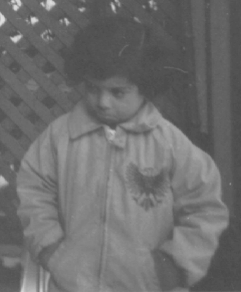
Remember when you saw that low-quality image and felt a bit disappointed? It wasn’t clear enough, and the details were a bit fuzzy. What if you could enhance that image to a better version? Wouldn’t that be great? Fortunately, there’s a way to do that, using Python!
One of the methods you can use to enhance an image is histogram equalization, which in particular enhances the contrast of the image. Almost all camera systems actually use histogram equalization to make our pictures look better, and at the end of the tutorial you will discover why this is so.
In the next section, I will delve deeper into what is meant by histogram equalization and what happens to the image when applying the method, and then we’ll see how we can implement the method in Python. Ready?
Histogram Equalization
Let’s say you have the pout.jpg image (go ahead and download it). This is a demo image used in MATLAB, where I got it from, but we will use it in our tutorial here. The image looks as follows:

Let’s take a look at how we can access the pixel values of the image, referred to as intensities. I wrote this small Python script that we can use to do just that (notice that I’m using the OpenCV library):
import cv2

img = cv2.imread('pout.jpg')
img_shape = img.shape
height = img_shape[0]
width = img_shape[1]

for row in range(width):
    for column in range(height):
		print (img[column][row])
What I’m doing here is reading our image (pout.jpg), and then investigating the shape (size) of the image. img_shape will return: (1031, 850, 3). This means that our image is of height (number of columns) 1031, and of width (number of rows) 850, and has 3 channels (RGB). Notice that the first parameter in the result is the height, and the second parameter is the width. Finally, we loop through the rows and columns and print out the different pixel values (intensities) at each row/column pair.
One sample of the output is: [137 137 137]. Yes, I know, you were expecting one value as a result for the pixel intensity. We actually have the value of the pixel intensity here, but what the output is showing us are the results of the red, green, and blue (RGB) channels. Please be aware, however, that in OpenCV the order is BGR, as this is how OpenCV loads the image. Thus, the above sample result contains the value 137 for each channel, in the order of B, G, and R, respectively.
The reason for the introduction is that histogram equalization is actually about the modification of pixel intensities for the sake of improving the image’s contrast. Thus, our main work here will be at the pixel intensity level.
At this point, you might be wondering what a histogram is. Although sometimes the term might be a bit confusing, it is actually a very simple concept. The histogram is simply a diagram that depicts the number of pixels in an image at each intensity value found in that image.
Since our pixels have three values, one for each of the BGR channels, one way to draw the histogram is to have three histograms, one for each channel, where the x-axis will have the different pixel values (intensities), and the y-axis will show how many times (frequency) that particular pixel value appeared among the different pixel values.
For instance, the red channel histogram can have a pixel value of 137 on the x-axis, and the y-axis can show how many pixels had this value for the red channel—say, for instance, 86. So the way we read that is by saying that the pixel value for the red channel of 137 showed up in 86 pixels, or has repeated 86 times in our image.
Using the code from this Image Histogram article to draw the histogram for our image, we get the following:

The histogram is actually for the red, green, and blue channels. Let’s take a small sample of the output you would get from the previous code, as shown below. This shows that the channel values seem to always be the same, and the different three lines drawn will thus have the same values and will be drawn on top of each other, appearing as only one line.
[94 94 94]
[95 95 95]
[97 97 97]
[99 99 99]
[100 100 100]
[101 101 101]
[101 101 101]
[101 101 101]
[100 100 100]
[98 98 98]
[95 95 95]
[93 93 93]
What the histogram equalization method will do for the above histogram is that it will transform the intensity values in a way that will make the histogram look flatter in the resulting image. In other words, histogram equalization is a method that adjusts image intensities in order to enhance the contrast of the image.
The above histogram looks a bit concentrated towards the middle of the figure, and what histogram equalization will do is distribute the pixel intensity values further to get a more flattened histogram.
I think that’s sufficient about histogram equalization to discuss here, as we don’t want to get more mathematical in this tutorial, especially since it is more about the implementation of the method in Python. However, you can check these notes that show the different formulas involved in the method: histogram equalization. So now let’s dive in to the implementation!
Histogram Equalization in Python
In this section, I will show you how to implement the histogram equalization method in Python. We will use the above image (pout.jpg) in our experiments. Let’s go through the process step by step. The first thing we need to do is import the OpenCV and NumPy libraries, as follows:
import cv2
import numpy
After that, we simply need to read our image, pout.jpg:
img = cv2.imread('pout.jpg')
The good news is that OpenCV provides us with a function through which we can apply histogram equalization on an image, namely equalizeHist(). It is straightforward to apply this function on a grayscale image as the method actually equalizes the histogram of a grayscale image, but in our case we have three channels (RGB) for each pixel and we cannot apply histogram equalization on the three channels in a separate manner.
A nice solution I came across in the book Python: Real World Machine Learning is to convert our image to the YUV color space, equalize the Y channel, and finally convert the result to RGB. So the first thing we do is convert our image to YUV. This can be done using the cvtColor() method, which converts the image from one space color to another, as follows:
img_to_yuv = cv2.cvtColor(img,cv2.COLOR_BGR2YUV)
Notice that we use BGR instead of RGB here, since OpenCV (as mentioned before) loads the images in BGR format.
We now apply the histogram equalization method on the Y channel using the equalizeHist() method:
img_to_yuv[:,:,0] = cv2.equalizeHist(img_to_yuv[:,:,0])
Finally, we convert the Y channel to RGB (BGR in OpenCV), as follows:
hist_equalization_result = cv2.cvtColor(img_to_yuv, cv2.COLOR_YUV2BGR)
Congratulations! You have now applied histogram equalization to the image. In the next subsection, I will put all the code together and show you how our image will look like after applying histogram equalization.
Putting It All Together
Let’s put everything we have learned together. The Python script for applying histogram equalization on pout.jpg looks as follows:
import cv2
import numpy

img = cv2.imread('pout.jpg')
img_to_yuv = cv2.cvtColor(img,cv2.COLOR_BGR2YUV)
img_to_yuv[:,:,0] = cv2.equalizeHist(img_to_yuv[:,:,0])
hist_equalization_result = cv2.cvtColor(img_to_yuv, cv2.COLOR_YUV2BGR)

cv2.imwrite('result.jpg',hist_equalization_result)
The output of the above script is the following image:

To notice the difference better, I will put the two images beside each other (left: original image; right: result of histogram equalization):

Did you notice the difference? The right image looks much clearer than the original image. No wonder why almost all imaging systems perform histogram equalization!
Before we wrap up, let’s see what the histogram of our result looks like:

If you compare the histogram of the resulting image with the histogram of the original image, you will notice that the histogram of the resulting image is flatter than the histogram of the original image, and this is exactly what the histogram equalization method does.
Conclusion
In this tutorial, we saw how we can enhance the contrast of an image using a method called histogram equalization, and how it is easy to implement using Python and OpenCV.
The result was very interesting as it was much clearer than the original image, and the histogram of the result was flatter than the histogram of the original image, showing a better distribution of pixel intensity values across the image.
Finally, don’t hesitate to see what we have available for sale and for study in the Envato Market, and please ask any questions and provide your valuable feedback using the feed below.
Powered by WPeMatico


